



It looks like a dartboard, a spider’s web or a bowl of coloured rings. It is actually the most useful picture in radio: one round chart that shows how well an antenna and its cable “agree” with the radio, and how to fix them when they do not. Here is that chart explained in plain language, panel by panel, with the instruments that draw it and the antennas it describes.
A story from the club field
(An illustrative story. The characters are fictional, and all numbers in this article come from standard formulas or from calculations shown below.)
Amir, who now has his 40 m beam on the drawing board, arrives at the club station with the infographic on his phone. “Pak Long, what is this? A target for archery? Everyone keeps posting it, and I nod politely.”
Pak Long laughs and fetches a small blue box with two sockets. “It is a target, you are not wrong. The bullseye is the centre, and it means everything the radio sends goes out of the antenna and nothing comes back. Every antenna lands somewhere on this chart. The further from the bullseye, the more signal is bounced back down the cable. The chart does not only tell you that you missed; it tells you which direction you missed in, so you know whether to add a coil, a capacitor, or a piece of cable.”
He connects a dipole, presses a button, and a yellow curve crawls across the little screen. Amir sees it pass near the centre at 7.1 MHz. “That is a good antenna,” says Pak Long. “And you can read that from one glance, with no calculator.” This article is what Amir wrote in his notebook afterwards.
What is the Smith chart, in one minute?
The Smith chart is a map of every possible impedance, folded into a circle so that “nothing” and “infinity” both fit on the page. Pick a spot on the map and it tells you the impedance, how much signal reflects, and how to get to the centre (a perfect match).
It was invented by Phillip H. Smith of Bell Telephone Laboratories, who published it in Electronics magazine in 1939 (references 1 and 2), long before pocket calculators. Engineers used a printed chart, a pencil and a compass to design matching systems for radar, telephone lines and broadcast antennas. The chart survived, because even with computers, the picture shows things that a column of numbers hides.
First, a few words in plain language
You do not need mathematics to follow the chart, but you do need seven words. Here they are, with everyday meanings:
| Word | Plain meaning | Symbol / unit |
|---|---|---|
| Impedance | How hard the antenna (or any load) “pushes back” against the signal. It has two parts: a resistance part and a reactance part. | Z, in ohms (Ω) |
| Resistance | The part that really uses up power: it becomes radio waves (good) or heat (bad). | R, in Ω |
| Reactance | The part that only stores energy and gives it back. A coil is “lazy” (current arrives late, +jX). A capacitor is “eager” (current arrives early, −jX). | X, in Ω |
| Characteristic impedance | The “road width” of the cable. Ham coax is normally 50 Ω; TV coax is 75 Ω. | Z0 (“Z-zero”) |
| Normalised impedance | The impedance divided by the cable’s. 50 Ω becomes 1, 100 Ω becomes 2, 25 Ω becomes 0.5. The Smith chart only uses these small numbers, so one chart fits every cable. | z = Z ÷ Z0 |
| Reflection coefficient | How much of the wave bounces back from the antenna. 0 means nothing bounces (perfect), 1 means everything bounces. | Γ (“gamma”), 0 to 1 |
| VSWR / SWR | The same reflection story told as a ratio that you read on a meter. 1:1 is perfect. | 1:1 to ∞ |
| Return loss | The same story again, in decibels: how many dB weaker the echo is than the original signal. Bigger is better. | dB |
Think of a garden hose connected to a tap. The hose has a certain “width” (the cable, 50 Ω). If the nozzle (the antenna) is just as wide as the hose, the water flows out smoothly. If the nozzle is much narrower or much wider, some of the water slaps back and sloshes along the hose. A radio wave in coax behaves the same way: the mismatch makes part of the wave echo back toward the radio. The Smith chart is how we measure the echo and decide which kind of adapter to add.
Reading the infographic, panel by panel
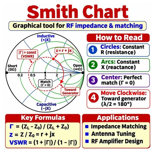
Now we can look at the picture at the top, step by step. The infographic has four numbered boxes on the right, then formulas and applications at the bottom.
Box 1: “Circles: constant R (resistance)”
The green circles all touch the right-hand edge. Each one is a fixed amount of resistance. The big circle through the centre is “1”, meaning 50 Ω on a 50 Ω chart. Circles further to the left (0.5, 0.2) are lower resistance (25 Ω, 10 Ω); circles to the right (2, 5) are higher (100 Ω, 250 Ω). Wherever your point sits, the circle passing through it tells you its resistance.
Box 2: “Arcs: constant X (reactance)”
The blue arcs curve away from the right-hand edge, some upward, some downward. The upward ones (+jX) are inductive, like a coil. The downward ones (−jX) are capacitive, like a capacitor. The straight line in the middle is the zero-reactance line: points on it are pure resistance, and the antenna is “resonant”. The infographic marks this with “Inductive (+jX)” at the top and “Capacitive (−jX)” at the bottom.
Box 3: “Center: perfect match (Γ = 0)”
The centre of the chart is z = 1: exactly 50 Ω and no reactance. Nothing bounces back, so Γ = 0 and the VSWR is 1:1. This is the bullseye and the goal of every matching job.
Box 4: “Move clockwise: toward generator (λ/2 = 180°)”
“Generator” means the radio. If you lengthen the cable, the impedance you see at the radio end rotates clockwise around the centre, at a constant distance from it. One full turn of the chart equals a cable half a wavelength long. The “180°” in the infographic is that same half-wavelength written as an electrical angle. We draw this in the walking figure later.
The dashed red circle: “|Γ| = const (VSWR)”
The red dashed circle around the centre in the infographic is the VSWR circle. Every point on one circle has the same VSWR. The nearer a circle is to the centre, the better the match. Note that the labels at the left and right edges, “Short (0 Ω)” and “Open (∞ Ω)”, are the two worst cases: a wire shorted at the end and a cable with nothing connected. Both reflect everything.
The three formulas
The bottom-left box of the infographic lists three formulas. They look scary but each one is simple arithmetic:
- Γ = (ZL − Z0) ÷ (ZL + Z0), the echo size. ZL is the antenna (the “load”) and Z0 is the cable. If the antenna is 100 Ω on a 50 Ω cable: (100 − 50) ÷ (100 + 50) = 50 ÷ 150 = 0.33. A 25 Ω antenna gives (25 − 50) ÷ 75 = −0.33, the same size, so it reflects exactly as much. Both are on the same VSWR circle.
- z = Z ÷ Z0 = r + jx, “normalising”: divide by the cable’s value so that one chart serves every cable. The antenna at 100 + j50 Ω becomes z = 2 + j1.
- VSWR = (1 + |Γ|) ÷ (1 − |Γ|), the number on your SWR meter. With |Γ| = 0.33: 1.33 ÷ 0.67 = 2.0, i.e. 2:1.
For a purely resistive antenna, the VSWR is simply the bigger of the two resistances divided by the smaller. A 100 Ω antenna on 50 Ω cable: 100 ÷ 50 = 2:1. A 25 Ω antenna: 50 ÷ 25 = 2:1. A 300 Ω folded dipole straight on 50 Ω: 300 ÷ 50 = 6:1.
The chart, with every part labelled
Here is the chart drawn from scratch with the same rules, and an example point marked: an antenna of 100 + j50 Ω on 50 Ω cable.
How to find the point, step by step. (1) Divide by 50: z = 2 + j1. (2) Find the green circle labelled “2” on the horizontal line. (3) Find the blue arc labelled “+j1”, the one that starts at the very top of the chart and curves to the right. (4) Where they cross is your point. (5) Read the echo from the red circle: it passes through the right half of the axis at 2.6, so the VSWR is 2.6:1. The echo size is |Γ| = 0.45.
That is it: two circles, one crossing, one answer. A printed chart has lots of tiny lines for the in-between values, but the idea never changes.
How the distance from the centre becomes the VSWR
Every point in the circle has a distance from the centre, and that distance is the echo size Γ. The edge of the chart is Γ = 1 (everything reflects), the centre is Γ = 0 (nothing reflects). So, to compare two antennas, look at which sits nearer the centre.
The table is the part worth remembering. A VSWR of 2:1 still delivers 89 % of the power to the antenna and the loss is only about 0.5 dB, far too small to hear at the other end. At 3:1, 75 % still gets through (about 1.2 dB lost). The practical problem is not the lost power but that many transmitters start to fold back their output somewhere between 2:1 and 3:1, and cable losses rise as the echo runs up and down the cable. A good aim for any antenna is a VSWR below 2:1 across the band you use.
Walking along the cable
Here is the idea behind the “clockwise” rule. We take the same 100 + j50 Ω antenna, connect cables of different lengths and look at what the radio sees.
The antenna did not change. The VSWR did not change (2.6:1 all the way, if the cable has no loss). Only the viewpoint changed. This is why an antenna analyser used at the shack end of a long cable can show reactance that is not in the antenna at all, and why the same antenna with a different cable length can make an old transceiver behave differently. Smart builders use this in reverse: a cable of the right length can turn an awkward impedance into a friendlier one. A quarter-wave cable flips a point to the opposite side of the chart, which is how a 75 Ω quarter-wave section can match a 100 Ω loop to 50 Ω coax.
The cable’s wavelength is shorter than in air. A coax with a velocity factor of 0.66 has a quarter-wave of 0.66 × (λ ÷ 4). For 7.1 MHz this is 0.66 × 10.6 m ≈ 7.0 m, not 10.6 m.
Matching an antenna: drawing the fix on the chart
This is the real power of the chart. Suppose a small antenna has an impedance of 20 + j15 Ω at 7.1 MHz. On the 50 Ω chart that is z = 0.4 + j0.3, point A. The VSWR is about 2.8:1. Two simple parts take us to the centre, and the chart tells us which ones and how big, without any algebra.
- Rule 1: adding a coil in series moves the point up, along the resistance circle (the green dashed one in the picture). A capacitor in series moves it down.
- Rule 2: adding a capacitor across the line (in parallel) moves the point along a circle that is the mirror image (the purple dashed one). A coil across the line moves it the other way.
The path goes from A up to B (series coil, about 213 nH at 7.1 MHz), then from B down into the centre (parallel capacitor, about 549 pF). In real life, you would use the nearest standard parts or a variable capacitor, adjust with the analyser watching, and enclose the network in a weatherproof box at the feed-point. This is exactly what an antenna tuner does, but automatically and with adjustable parts. It is also what a gamma match, hairpin match and L-network are, in different mechanical dress.
The matching network makes the radio and the cable happy, but it does not make a poor antenna radiate better. An antenna tuner in the shack hides the mismatch from the transmitter, but the echo still bounces up and down the cable and heats it. Always fix the problem as near to the antenna as possible.
What equipment produces the chart?
The instrument is called a vector network analyser, or VNA. “Vector” means it measures both the strength and the timing of the echo, which is exactly what you need to place a point on the chart. Fortunately, the old lab-sized instrument now has a hand-held cousin that costs far less and fits a shirt pocket.
Inside the box, there are four small jobs: a signal source sweeps through the band; a bridge or coupler separates what goes out from what comes back; a receiver measures both; and a chip divides one by the other to find Γ. From Γ it can calculate R, X and the VSWR and draw the chart. The yellow curve in the picture is our own calculated 40 m Yagi sweep (explained in the Yagi figure further down). Here are the usual options:
| Instrument | What it is | Who uses it |
|---|---|---|
| Vector network analyser (VNA), hand-held, e.g. the NanoVNA family | A small battery-powered box with two ports and a screen. It sweeps a band, measures the reflection and draws the Smith chart, VSWR and R + jX. Many also talk to a PC or phone. | The hobby standard today: low cost, light enough to carry up a mast. |
| Antenna analyser (older style) such as the MFJ-259 or RigExpert types | Same idea, built for antennas. Some show only numbers (R, X, VSWR); newer ones plot the chart. | Radio amateurs tuning antennas in the field. |
| Bench VNA from lab-instrument makers | A large, accurate instrument with a wide frequency range and a careful calibration kit. | Laboratories and manufacturers. |
| Antenna-modelling software (e.g. 4nec2 and similar) | No hardware at all: the computer calculates the impedance of a drawn antenna and plots it on a Smith chart. | Designers who want to check an antenna before cutting metal. |
| Matching-design software (e.g. SimSmith, Smith V4, scikit-rf in Python) | Lets you add coils, capacitors and cable pieces on screen and watch the point move to the centre. | Anyone designing a matching network. |
How to measure properly
- Calibrate first with the three standards in the picture: short, open, load. The analyser learns what “zero” and “infinity” and “perfect” look like, and corrects itself. Calibrate with the same cable you will measure through, at the end of that cable.
- Measure at the antenna, or compensate for the cable length. The analyser can do this with the “electrical delay” or “port extension” setting. Otherwise, you read the rotated chart that we walked in the previous section.
- Keep the outside of the coax out of it. A ferrite choke or 1:1 balun near the feed-point stops current flowing on the outer braid, which would otherwise distort the reading.
- Disconnect from the radio first. A hand-held VNA is not built for transmitter power. A long wire can also carry static or pick up strong broadcast signals, so touch the connector to ground before you plug it in.
- Sweep the whole band, not a single frequency. The curve is much more informative than a number.
What types of antenna does it describe?
All of them. The chart does not care what the antenna looks like: a dipole, a vertical, a beam, a loop or a bent coat hanger, all of them end up as a point (at one frequency) or a curve (over a band). Different antennas simply land in different regions, as shown here:
| Antenna | Typical feed-point impedance | Where it sits on the chart | How it is usually matched |
|---|---|---|---|
| Half-wave dipole, up in clear air | about 73 Ω (50–70 Ω when low over ground) | Slightly right of centre | Usually fed directly; a 1:1 current balun keeps the coax from radiating. |
| Inverted-V dipole | about 50 Ω | Right at the centre | The easy case: direct feed, plus a choke balun. |
| Quarter-wave vertical with radials | about 36 Ω (closer to 50 Ω if the radials droop) | Left of centre | Often fine as it is; drooping radials raise the value toward 50 Ω. |
| 3-element Yagi | about 20–35 Ω (our 40 m model: 34 Ω) | Well left of centre | Gamma, hairpin or beta match, or accept a VSWR of 1.5:1 as in our 40 m article. |
| Folded dipole | about 300 Ω | Far right | A 4:1 balun brings it to about 75 Ω, which is close enough to 50 Ω. |
| Full-wave loop (quad) | about 100–120 Ω | Right of centre | A quarter-wave section of 75 Ω cable, or a 2:1 transformer. |
| End-fed half-wave wire | 2,000–4,000 Ω or more | Right at the edge, near “open” | A 49:1 or 64:1 transformer at the feed-point. |
| Short whip or mobile antenna | a few Ω with a large −jX | Bottom half, far from the axis | A loading coil adds +jX and walks the point up to the axis; then raise the resistance. |
| Random wire | anything, and it changes with frequency | Scattered all over | An antenna tuner at the feed-point does the matching for you. |
The pattern is useful: the left half of the chart is “low resistance”, the right half is “high resistance”, the top is “too much coil”, the bottom is “too much capacitor”. The right fix always follows from where you landed. A transformer or balun moves a point left or right (it changes the resistance without adding reactance), while a coil or capacitor moves it up or down.
A real example: our 40 m Yagi
In our companion article on the 3-element 40 m Yagi, we calculated the antenna’s impedance across the band. Here is the same data, drawn on the Smith chart:
The curve answers in one picture what a table would need seventeen rows to say: the match is best near 7.0 MHz, where the curve passes closest to the centre (VSWR about 1.4:1). Above 7.12 MHz it leaves the orange 2:1 circle, because the antenna starts to look inductive. If the builder wants the best match nearer 7.1 MHz, trimming the elements a little shorter moves the best-match point up the band, and a new sweep shows how far you have gone.
Common mistakes and myths
- “Low SWR means a good antenna.” No. A dummy load has a perfect 1:1 and radiates nothing. The chart shows the match, not the radiation. A good match plus a good antenna design is what you want.
- “I measured 1.2:1 in the shack, so the antenna is fine.” A lossy or very long cable hides a mismatch by absorbing the echo. A poor antenna on a long thin cable can show a pretty chart because the cable is eating the signal.
- “The chart rotates when I change the cable, so my antenna changed.” No. It changes the view, not the VSWR.
- “I need 1.0:1.” No. Anything under 1.5:1 is very good for amateur work, and 2:1 is acceptable for most transmitters.
- “It only works at one frequency.” The chart shows one frequency as a point. A sweep gives a curve, and the curve is the full story.
Cheat sheet
- Centre = perfect (50 Ω, VSWR 1:1). Edge = total reflection.
- Top half = inductive (+jX, too much coil). Bottom half = capacitive (−jX, too much capacitor).
- Left = low resistance. Right = high resistance. Horizontal line = pure resistance (resonant).
- Distance from the centre = how much bounces back. One circle = one VSWR.
- Clockwise = toward the radio. One full turn = half a wavelength of cable.
- Series part = walk along a resistance circle. Parallel part = walk along the mirror-image circle.
- Calibrate (short, open, load), then sweep the band, and read the curve.
Try it yourself
Borrow or buy a hand-held VNA, calibrate it, and measure your own dipole from 6.9 to 7.3 MHz. Mark where the curve crosses the horizontal line (that is the resonant frequency). If it crosses below the frequency you want, the antenna is too long; if above, too short. Trim a few centimetres, sweep again, and watch the curve move. Ten minutes of that will teach you more than ten pages of text.
References and further reading
- Smith, P. H. “Transmission Line Calculator.” Electronics, vol. 12, January 1939. The paper that introduced the chart; Smith worked at Bell Telephone Laboratories.
- Smith, P. H. “An Improved Transmission Line Calculator.” Electronics, vol. 17, January 1944. The version that became the standard chart.
- Smith, P. H. Electronic Applications of the Smith Chart in Waveguide, Circuit, and Component Analysis. McGraw-Hill, 1969. The author’s own book, still reprinted.
- Pozar, D. M. Microwave Engineering, 4th ed., Wiley, 2012. Chapter 2 explains reflection, VSWR and the Smith chart with the mathematics.
- ARRL. The ARRL Antenna Book (current edition). Feed-point impedances, baluns, matching networks and antenna measurement. https://www.arrl.org/arrl-antenna-book
- Balanis, C. A. Antenna Theory: Analysis and Design, 4th ed., Wiley, 2016. Input impedance of dipoles, loops and arrays.
- “Smith chart.” Wikipedia, a good free overview with the construction of the circles. https://en.wikipedia.org/wiki/Smith_chart
- NanoVNA-Saver, free open-source PC software for NanoVNA-type analysers (Smith chart, VSWR and logging). https://github.com/NanoVNA-Saver/nanovna-saver
- The infographic at the top of this article was shared on Facebook. Original post: https://www.facebook.com/arashad.mohamed.50/posts/pfbid0q6t8j9LTkrtneMBbsk8w8s9Yx68QTs86rN1PaKEABpZt94Wynt2sd9TVVPvQEb6kl
The diagrams in this article are original JASRA drawings, computed from the chart’s standard equations. The sweep in the Yagi figure was calculated by JASRA for the drawing dimensions in the 40 m Yagi article. The story and its characters are fictional. The infographic at the top is shared for educational purposes; the original creator is not named beyond the link given in the references. This article is a learning guide: always disconnect an analyser from a transmitter before measuring, and follow safety rules when working on antennas.


